:::info This paper is available on arxiv under CC BY-SA 4.0 DEED license.

Authors:

(1) Lana L. Blaschke, Earth System Modelling, School of Engineering and Design, Technical University of Munich, Munich, Germany, Potsdam Institute for Climate Impact Research, Potsdam, Germany and [email protected];

(2) Da Nian, Potsdam Institute for Climate Impact Research, Potsdam, Germany;

(3) Sebastian Bathiany, Earth System Modelling, School of Engineering and Design, Technical University of Munich, Munich, Germany, and Potsdam Institute for Climate Impact Research, Potsdam, Germany;

(4) Maya Ben-Yami, Earth System Modelling, School of Engineering and Design, Technical University of Munich, Munich, Germany, and Potsdam Institute for Climate Impact Research, Potsdam, Germany;

(5) Taylor Smith, Institute of Geosciences, University of Potsdam, 14476 Potsdam, Germany;

(6) Chris A. Boulton, Global Systems Institute, University of Exeter, EX4 4QE Exeter, UK ;

(7) Niklas Boers, Earth System Modelling, School of Engineering and Design, Technical University of Munich, Munich, Germany, Potsdam Institute for Climate Impact Research, Potsdam, Germany, Global Systems Institute, University of Exeter, EX4 4QE Exeter, UK, and Department of Mathematics, University of Exeter, EX4 4QF Exeter, UK.

:::

Table of Links

• Abstract and Introduction
• Materials and Methods
• Data
• Results
• Conclusions, Open Research Section and Conflict of Interest/Competing Interests
• Author Contributions, Supplementary Information, Acknowledgments and References
• Additional Insight from the Conceptual Model
• AMSR2 until 2022 Excluded Due to Missing Human Land Use Data
• Investigation of Resilience Loss in AMSR2’s X-Band
• Results Proving Robustness
• Potential Driving Forces and Sources of Bias

RESULTS PROVING ROBUSTNESS

Text S8. Robustness with respect to the parameterization of the STL algorithm

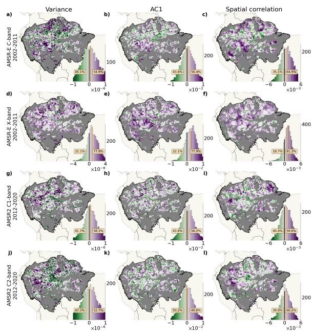
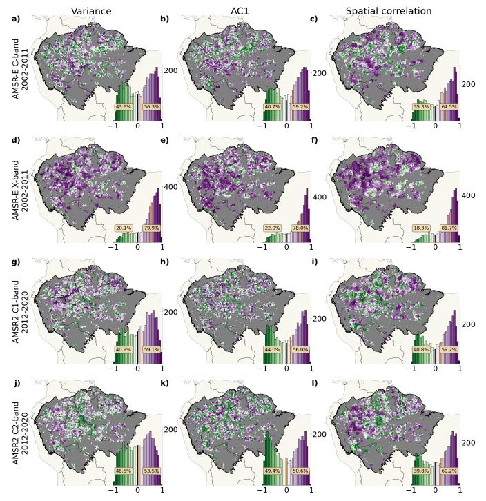
The results in Figures 5 and 6 are based on the residual found by the STL algorithm with default parameterization. Yet, Figure S9 and S10 prove that the analysis is not influenced by this choice as the results are almost identical when the length of the seasonal smoother equals 13 (instead of 7).

Text S9. Robustness with respect to the size of the sliding windows

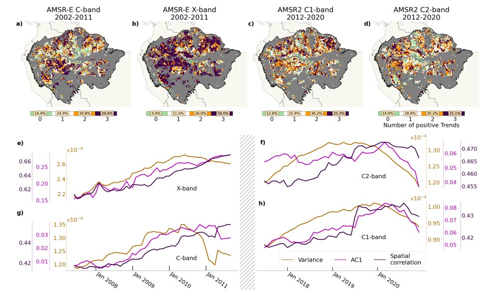
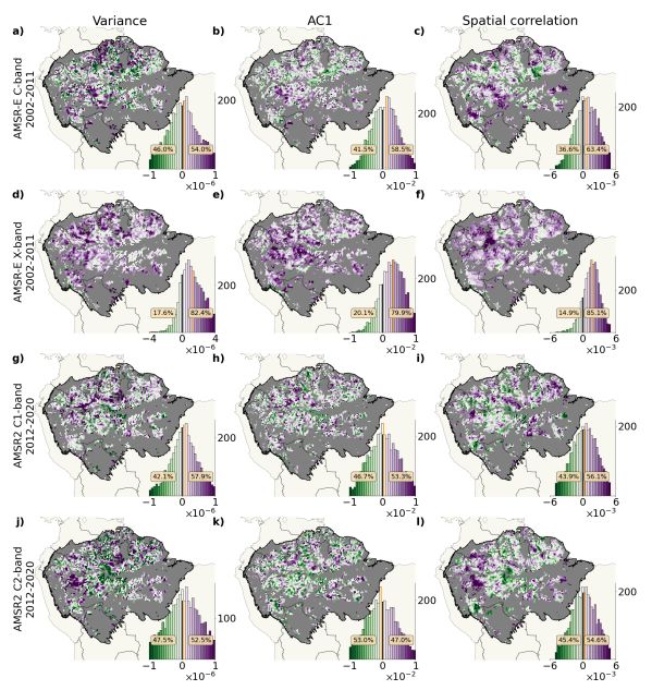
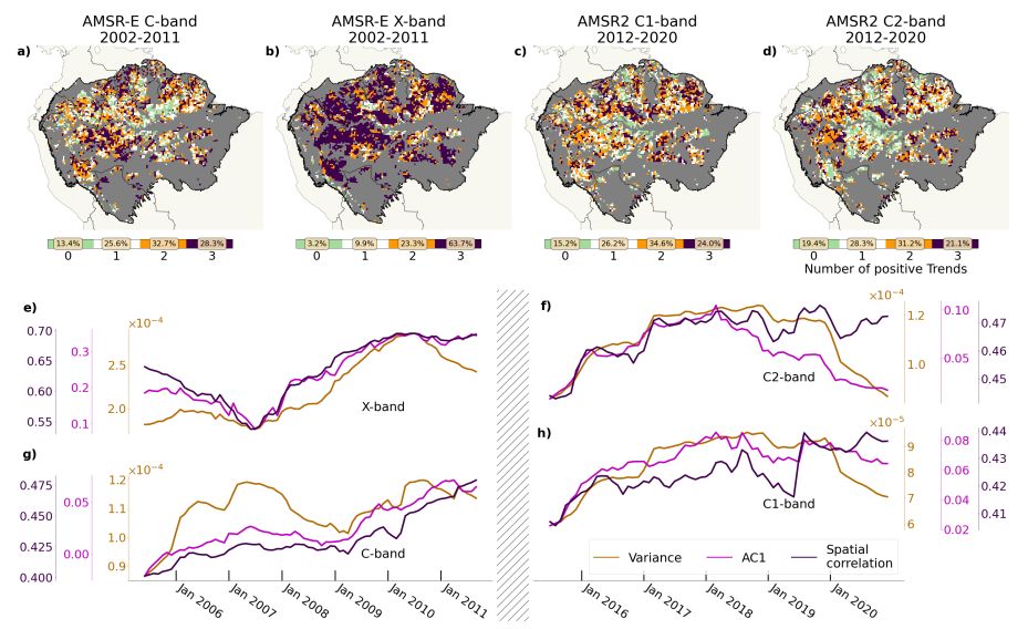
The choice of the sliding window size is difficult for short time series as that of AMSR-E’s and AMSR2’s VOD. Yet, the results are robust w.r.t it, as Figure S11 based on sliding windows of 3 years is almost identical to Figure 5 with windows of 5 years. This also holds for the summarizing Figure S12 when compared to Figure 6. It is to note that the spatially averaged time series of the three indicators are more noisy for the choice of smaller windows, which is due to the fact the the calculation of the indicators becomes more unstable when calculated on only 36 data points, corresponding to the 3 years. The right choice of the window size in an approach to resilience analysis like the one shown here is challenging, as the increase can only be determined reliably based on enough indicator time steps either. The fact that the results are robust with respect to the window size gives confidence in the choice of 5 years as default.

Text S10. Robustness with respect to the measure of change

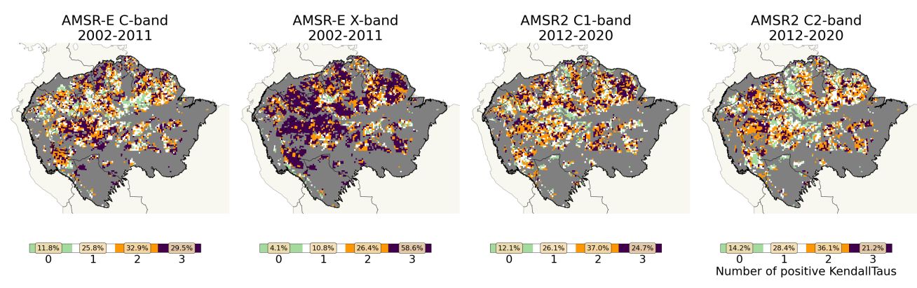
In the main text, any change in indicators is measured in terms of linear trends. Yet, another option would be the Kendall’s τ as a measure of steadiness of increase. Figure S13 is the analogue of Figure 5 but with increase in time series quantified in terms of Kendall’s τ . In Figure 6, increase in the indicators is quantified in terms of linear trends. The results are almost identical when measuring the indicators’ increase by the Kendall τ rank coefficient.

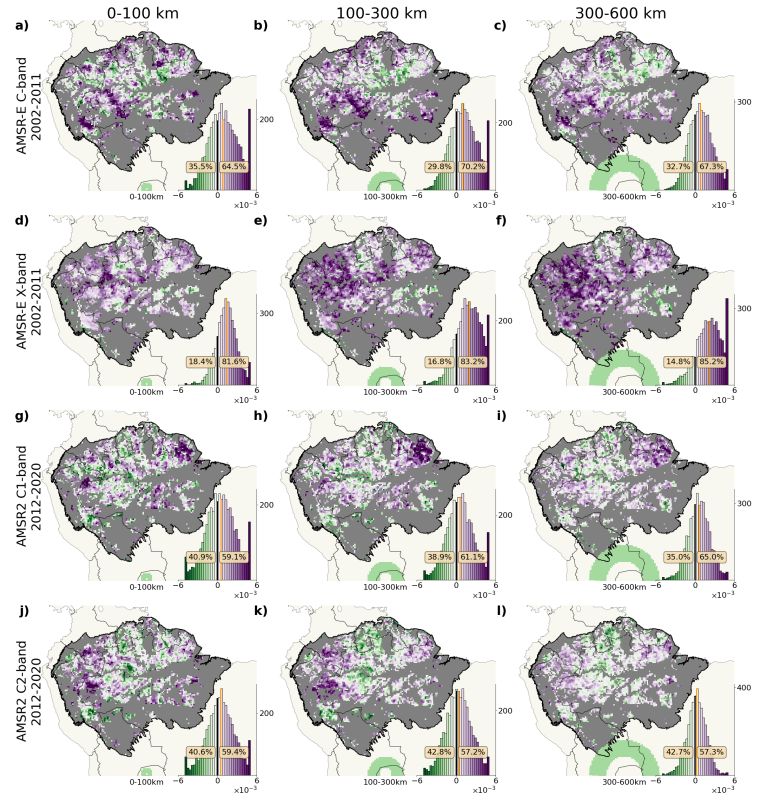
Text S11. Robustness with respect to the distance defining neighboring cells

The definition of the spatial correlation depends on the distance taken into account when taking the average correlation with neighboring cells. Figure S15 shows the trends of the spatial correlation for the different VIs comparing different radii defining the set of neighboring cells. As expected, a greater number of neighbors spatially smooths the results, but does not influence the general spatial pattern of the trends of spatial correlation. The turquoise circle on the bottom of the map shows an exemplary circular band of neighboring cells. In the main text, all results are based on a radius of 100 km.

\

\

\

\

\

\

\