:::info This paper is available on arxiv under CC BY-SA 4.0 DEED license.

Authors:

(1) Lana L. Blaschke, Earth System Modelling, School of Engineering and Design, Technical University of Munich, Munich, Germany, Potsdam Institute for Climate Impact Research, Potsdam, Germany and [email protected];

(2) Da Nian, Potsdam Institute for Climate Impact Research, Potsdam, Germany;

(3) Sebastian Bathiany, Earth System Modelling, School of Engineering and Design, Technical University of Munich, Munich, Germany, and Potsdam Institute for Climate Impact Research, Potsdam, Germany;

(4) Maya Ben-Yami, Earth System Modelling, School of Engineering and Design, Technical University of Munich, Munich, Germany, and Potsdam Institute for Climate Impact Research, Potsdam, Germany;

(5) Taylor Smith, Institute of Geosciences, University of Potsdam, 14476 Potsdam, Germany;

(6) Chris A. Boulton, Global Systems Institute, University of Exeter, EX4 4QE Exeter, UK ;

(7) Niklas Boers, Earth System Modelling, School of Engineering and Design, Technical University of Munich, Munich, Germany, Potsdam Institute for Climate Impact Research, Potsdam, Germany, Global Systems Institute, University of Exeter, EX4 4QE Exeter, UK, and Department of Mathematics, University of Exeter, EX4 4QF Exeter, UK.

:::

Table of Links

• Abstract and Introduction
• Materials and Methods
• Data
• Results
• Conclusions, Open Research Section and Conflict of Interest/Competing Interests
• Author Contributions, Supplementary Information, Acknowledgments and References
• Additional Insight from the Conceptual Model
• AMSR2 until 2022 Excluded Due to Missing Human Land Use Data
• Investigation of Resilience Loss in AMSR2’s X-Band
• Results Proving Robustness
• Potential Driving Forces and Sources of Bias

\

ADDITIONAL INSIGHT FROM THE CONCEPTUAL MODEL

Text S1. Stability in the conceptual model

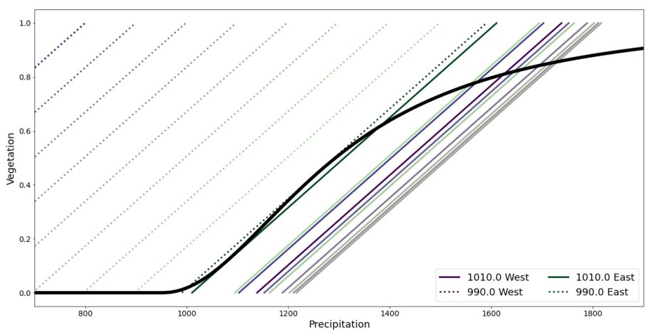
The interaction of vegetation and precipitation is plotted in Figure S1. In the conceputal model, vegetation is a function of absolute incoming precipitation only and is not dependent on the cell’s location. Hence, it is the same for each cell and plotted as the single black solid line. Precipitation on the other hand is a function of the vegetation of the cell, but also of the vegetation of the cell’s eastern neighbors. Hence, it differs for all cells, which are encoded by the colors as in Figure 2. For the calculation of one cell’s precipitation as a function of vegetation, its eastern neighbors are considered to be in equilibrium. Furthermore, precipitation depends on the amount of moisture coming in from the Atlantic ocean, or in other words on the control parameter B. The solid lines represent the state in the beginning of the experiment with B = 1010, and the dashed lines in the end with B = 990. Where the black and coloured lines cross at some (V∗, P∗), the corresponding value of vegetation supports the value of precipitation P∗, but also is V∗ supported by P∗. Hence, this point is considered a fixed point, or equilibrium. As the moisture inflow is reduced in the simulations from 1010 (solid lines) to 990 (dashed lines), the fixed points with high vegetation values vanish, explaining the tipping in the Figures S4 and S5 .

Text S2. Precipitation decrease in the conceptual model

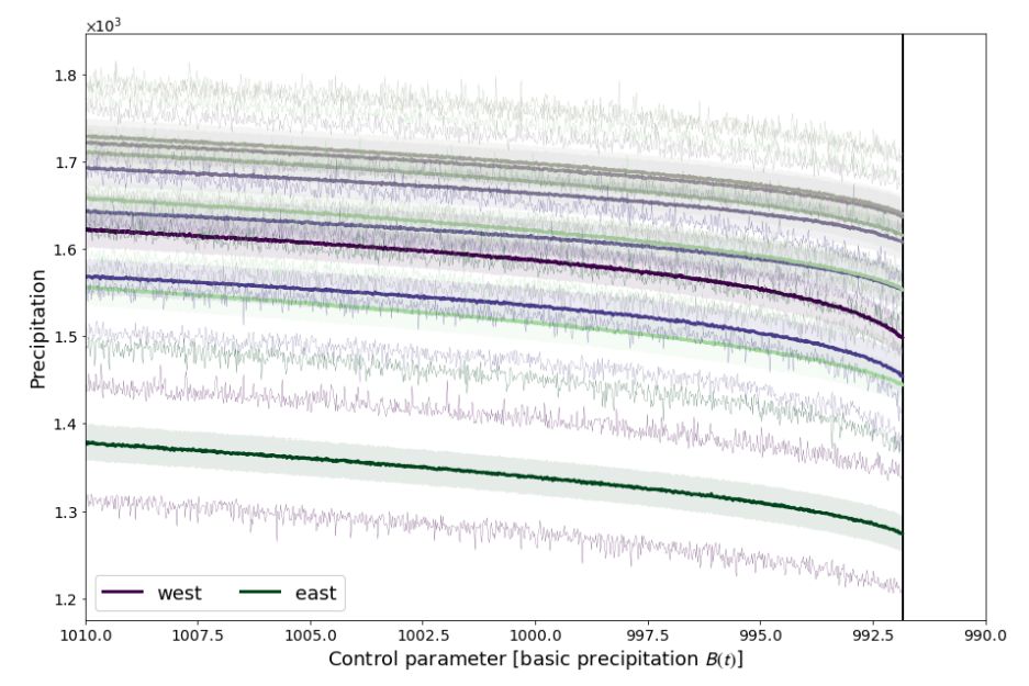
The results of simulations with decreasing moisture inflow from the Atlantic ocean (decreasing B(t)) were presented in the main text in Figure 4. Figure S2 zooms in into cell-wise total precipitation and highlights its stochasticity as well as the almost linear decrease up to the Tipping Point of vegetation.

Text S3. Deforestation scenario leads to Tipping in the conceptual model

The results of simulations with decreasing moisture inflow from the Atlantic ocean (decreasingB(t)) were presented in the main text in Figure 4. Figure S3 is identical but presents the results from simulations with unchanging inflow from the Atlantic, i.e. B(t) = 1000 for all t. Instead, the amount vegetation in the east-most cell is considered the bifurcation parameter and constantly decreased from 1 to 0, thereby mimicking deforestation.

Text S4. Distribution of the trends for the three resilience indicators

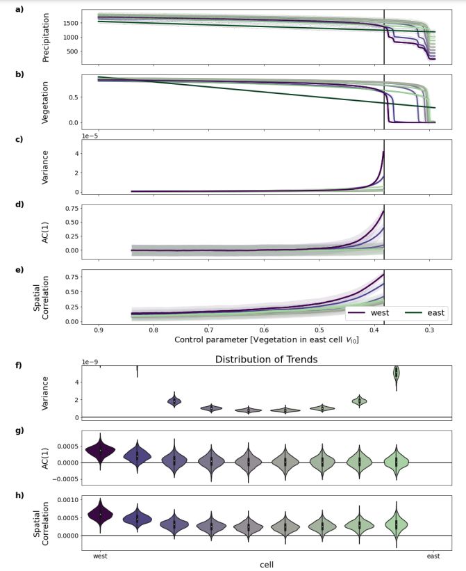
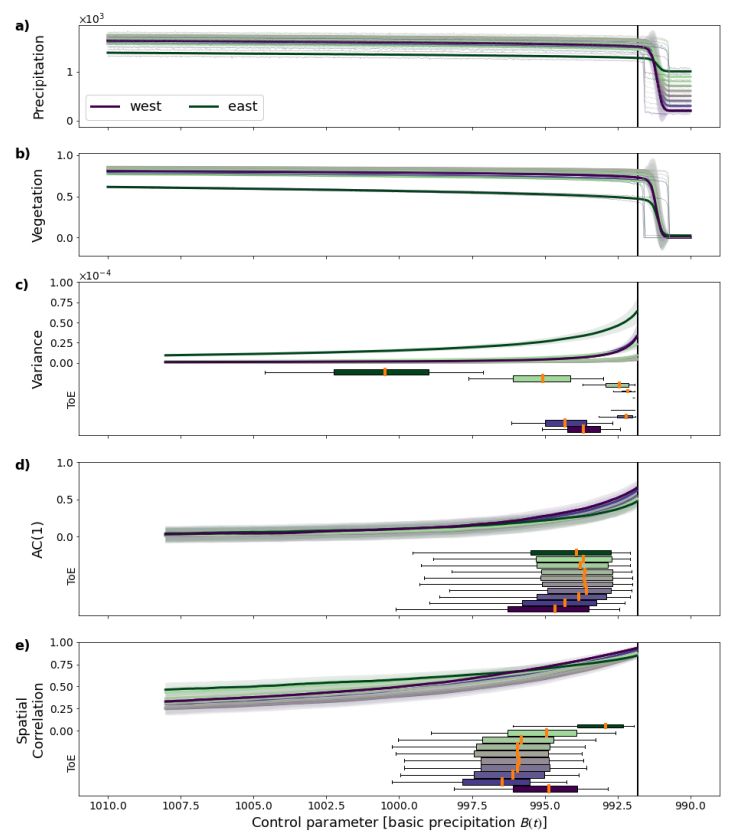
In the conceptual model, all indicators show clear trends when approaching the Tipping Point of vegetation, as illustrated in Figure S4. There, clearly all three indicators show a strong shift

\

\

\

\ towards positive values with only very few negative ones for AC1. In a spatially extended system like the ARF, one would thus expect all three indicators to increase when the corresponding grid cell loses resilience.

Text S5. Distribution of the trends for the three resilience indicators

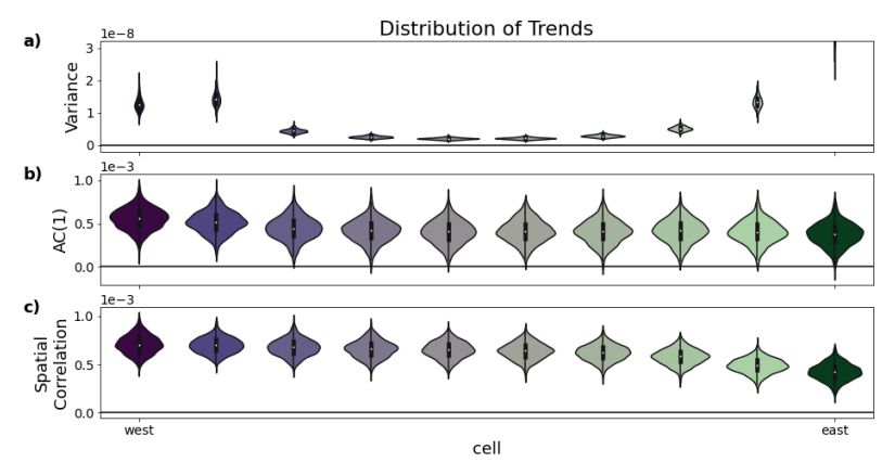
In Figure 4 the time of emergence (ToE) was defined as the first time when a trend becomes significant. Yet, as more conservative approach one can define the ToE as the time when a trend becomes permanently significant, i.e. when all trends later in time are significant as well. The results with this definition are displayed in Figure S5. The uncertainty in the timing of this type of ToE differs much less for AC1 compared to the definition in the main text. This indicates that AC1 might be more prone to false alarms.

\