:::info Authors:

(1) Jonathan H. Rystrøm.

:::

Table of Links

Abstract and Introduction

Previous Literature

Methods and Data

Results

Discussions

Conclusions and References

A. Validation of Assumptions

B. Other Models

C. Pre-processing steps

B Other Models

B.1 Model without activity-level

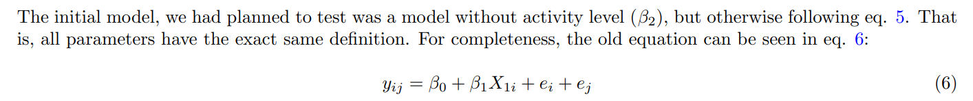
\ However, when we ran the model (also using lmerTest (Kuznetsova et al., 2017)) and plotted the residuals, we got the following:

\

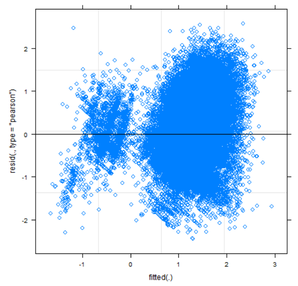
\ Just from a brief visual inspection, it is clear to see that the residuals are not randomly distributed: There are two distinct ”bands” that both seem to trend upward. This breaks the assumption that the residuals are randomly distributed (Poole & O’Farrell, 1971). While many assumption violations are reduced with enough data (Baayen et al., 2008; Schielzeth et al., 2020), non-linearity is not one of them (Poole & O’Farrell, 1971).

\ Fortunately, the non-random residuals were (partially) fixed by introducing activity-level for the reasons described in section 3.3.

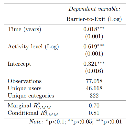
B.2 Problematic Categories Removed

Here we fit the main model (eq. 5, with problematic categories removed. We define a problematic category as a category with a fitted random effect of less than -0.5. We obtain this threshold by visually inspecting Fig. 7.

\ The results of this fit can be seen below in 2:

\

\

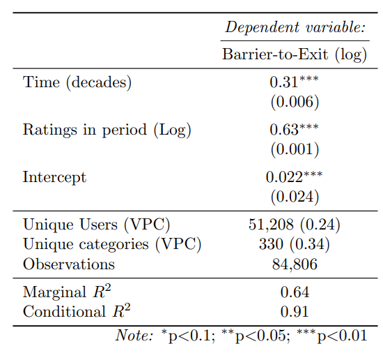
B.3 Gamma mixed-effects model

In the following, we refit the main model (eq. 5) using a Gamma regression. This is the most widely recommended solution in the literature on fitting right-tailed, heteroscedastic outcomes (Feng et al., 2014; Villadsen & Wulff, 2021).

\ However, since we discovered this after running our initial models, we could only justify doing this as a post-hoc test.

\ I use the lme4-package to fit the model (Bates et al., 2014). To avoid convergence errors and adapt the model to the formula, we make the following alterations:

\

1. Add a gamma log-link function (Fox, 2015)

   \

2. change the year (β1) estimate to decades. This has the effect of rescaling the effect size.

   \

3. We still log-transform the activity-level to rescale it. As this is not part of the hypothesis, this does not affect our interpretation.

\

\

\

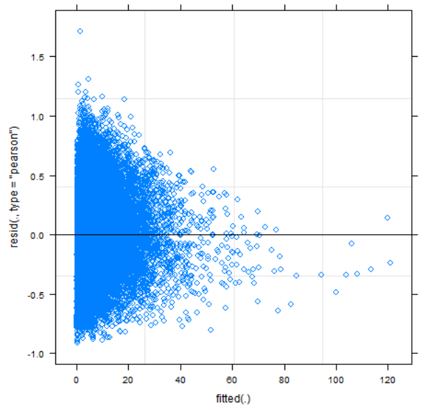
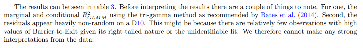
\ This leads us to the interpretation. The effect size per decade is 0.31, which is highly significant (SE=0.006, T=24, p ≪ 0.001). This translates into 34% increase per decade or 3% increase per year. This is the same direction as our transformed linear model, with somewhat larger results. However, as these come from an almost unidentifiable fit with extremely non-random residuals, no inferences can be drawn from this.

\ Some of this indicates that the conditional distribution of Barrier-to-Exit is not a Gamma distribution. Pursuing the GLMM path would require further assessments of the best-fitting distribution. This could be by e.g. applying the Box-Cox method as described by Villadsen and Wulff (2021).

\

:::info This paper is available on arxiv under CC 4.0 license.

:::

\