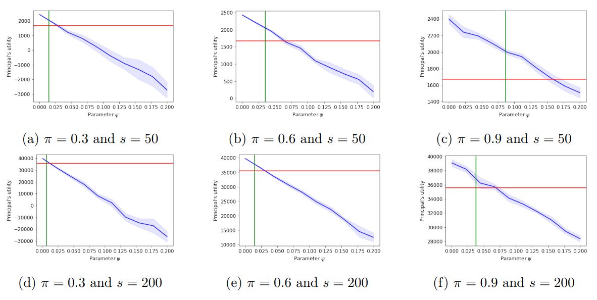
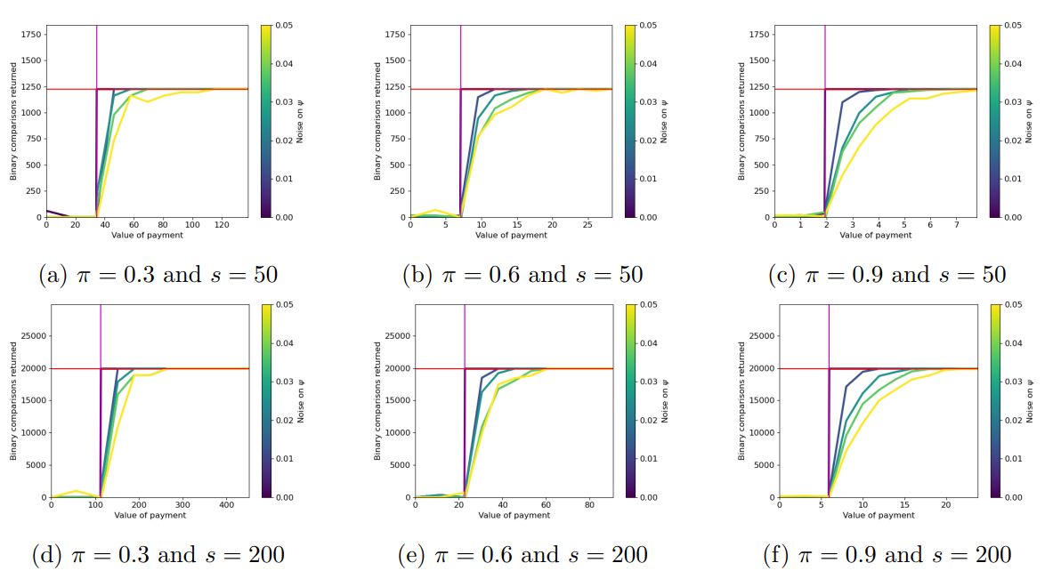
 Psst! Do you accept cookies?
:::info This paper is available on arxiv under CC 4.0 license.
Authors:
(1) Kiriaki Frangias;
(2) Andrew Lin;
(3) Ellen Vitercik;
(4) Manolis Zampetakis.
:::
Table of Links
Warm-up: Agents with known equal disutility
Agents with unknown disutilites
Conclusions and future directions, References
B Omitted proofs from Section 2
C Omitted proofs from Section 3
D Additional Information about Experiments
D Additional Information about Experiments
D.1 Post-processing algorithm
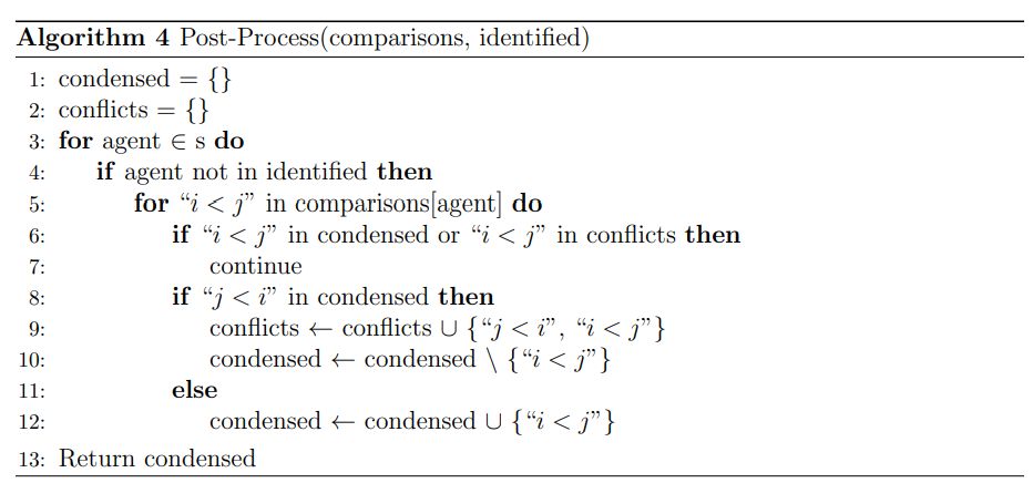
\ Algorithm 4 takes as input “comparisons”, which is a list of s sublists, each containing the returned results of the binary comparisons performed by an agent. Each result is represented with a string of the form “i < j”, representing that according to the agent, the true score of item Ti is smaller than that of item Tj. The input “identified” is a set containing the indeces of all agents who returned at least one verified comparison incorrectly.
\ Algorithm 4 iterates through the comparisons returned by agents not in the set “identified” and adds them to the set “condensed”, which will be returned at the end. If the comparison is already in the set “condensed”, then it is not added again. If there has been another agent whose returned comparison disagrees with it, then the comparison is added to the set “conflicts” (if not already added), and is removed from the set “condensed”.
\

D.2 Principal’s utility vs. parameter π
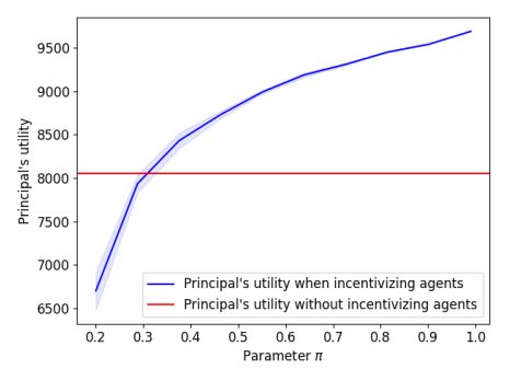
The plot shows a monotonic increase in the principal’s utility as π increases. The shaded region corresponds to a 90% confidence interval across 15 iterations. We notice that for any value of π that is greater than 0.35, it is in the principal’s best interest to implement our contract instead of performing all pairwise comparisons herself.
\
D.3 Additional Hyper-parameter settings from Section 4
For the remainder of this section, we fix the hyper-parameter settings found in Section 4, unless otherwise stated. Namely, we assume that π = 0.8, δ = 0.01, n = 100, s = 100, ψ¯ = 2, and ψ = 0.01.
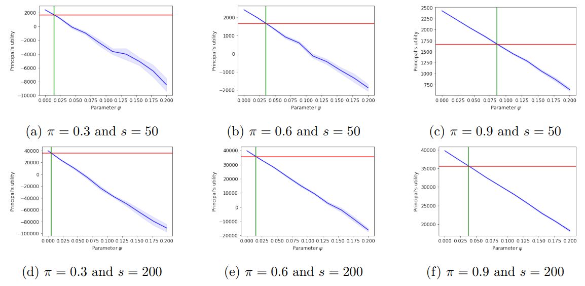
\ Discussion of Figure 5. In Figure 5 we provide additional hyper-parameter settings for Figure 1a in Section 4. First, we select the probability of an effortful agent being “good” to be a value in {0.3, 0.6, 0.9} and the number of agents and items to be in the set {50, 200}. In plots 5a-5c results are averaged across 15 trials, while in plots 5d- 5f, results are averaged across 10 trials.
\ The blue shading corresponds to a 90% confidence interval. We notice that the confidence intervals decrease with the number of agents, even for a small number of trials. The confidence intervals also decrease, as the agents’ work becomes more predictable (π increases).
\ We find that as π increases, the principal’s utility also increases along with the threshold for ψ, below which it is in the principal’s best interest to run CrowdSort than perform all comparisons herself. This threshold also decreases with the number of agents, s. This implies that there is a sweet spot, in which the expected number of “good” agents is just enough that the ground-truth ordering of the items is retrieved and it is sufficiently small so that the principal can pay all of them.
\
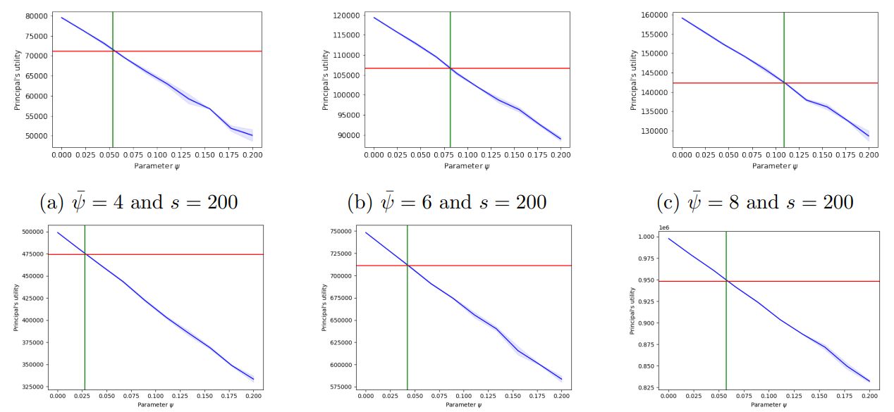
\ Discussion of Figure 6. In Figure 6 we provide additional hyper-parameter settings for Figure 1a in Section 4. Specifically, we select the per-comparison disutility of the principal, ψ¯, along with the per-comparison utility of the principal, λ, to take values in {4, 6, 8}. The number of agents and items is in the set {200, 500} and our results are averaged across 2 trials with the blue shading corresponding to a 90% confidence interval.
\ We notice that the utility of the principal dramatically increases with the value she assigns to the correct ordering. Interestingly, by comparing Figure 5f to Figures 6a-6a, we find that even when the reliability of the agents is smaller (π = 0.8 in 5f and π = 0.9 in 6a6c), the principal’s point of indifference is higher when her disutility is larger. As before, we notice that when a large number of agents is incentivized, their labor needs to be sufficiently inexpensive (smaller threshold on ψ) for their work to be more profitable to the principal than performing all pairwise comparisons herself.
\ Lastly, our results show, that for a broad range of hyperparameters, our theoretical analysis accurately predicts the value of ψ, for which the principal is indifferent between running CrowdSort or performing all comparisons herself.
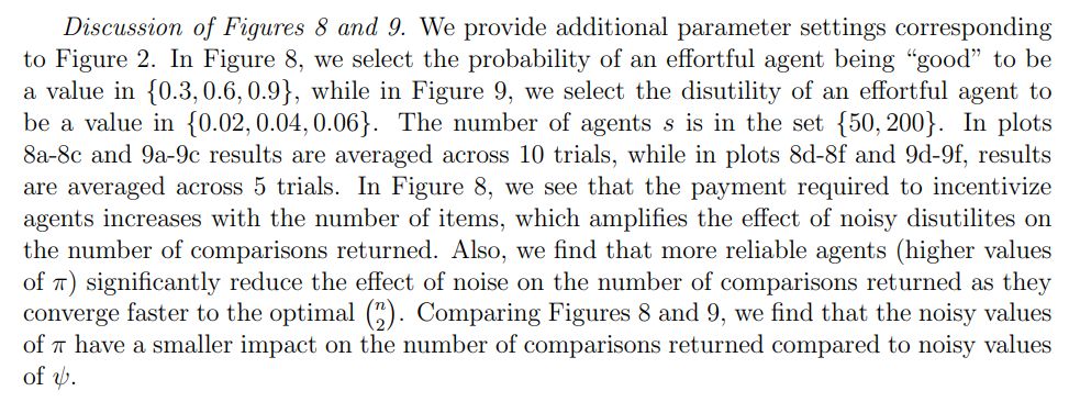
\ Discussion of Figure 7. We provide additional parameter settings corresponding to Figure 1b. The parameters π and s along with the number of trials vary as in Figure 5. We find that as the number of agents to be incentivized grows, our theoretical analysis for the principal’s point of indifference becomes more accurate.
\ Also, noise on the disutilites results in many agents not being incentivized to exert effort and therefore get paid. This increases the principal’s utility, especially when parameter π is large, therefore resulting in a less steep slope. As in Figure 1b, we note that the confidence intervals become larger with ψ, as the principal’s utility shows higher variance, when less agents are “good”.
\
\
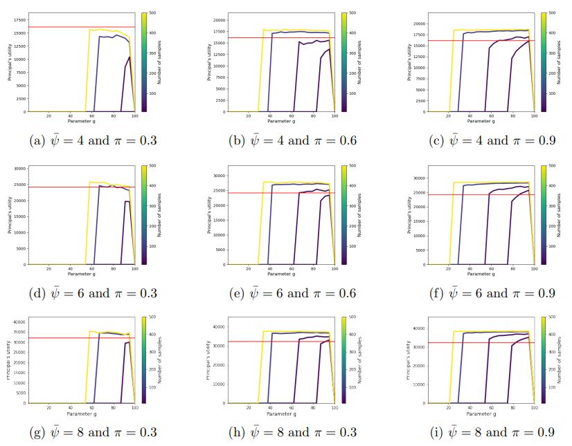
\ Discussion of Figure 10. In Figure 10 we offer a range of parameters corresponding to Figure 3 in Section 4. Specifically, we vary the probability than an effortful agent is “good”, which take values in {0.3, 0.6, 0.9} and the principal’s per-comparison disutility, ψ, and utility λ, which takes values in {4, 6, 8}. The multicolored plots indicate the principal’s utility for different sample sizes (namely, 10, 20, 100, and 500) drawn from D, which in this case is N (0.03, 0.01).
\ Notice that we do not normalize the y-axis in this case. Results are averaged across 10 trials.
\ We see that as agents become more reliable (higher value of π) and as the principal’s value for the correct sorting grows (λ), it becomes increasingly beneficial to the principal to run CrowdSort, than perform all pairwise comparisons on her own. Interestingly, even if π is 0.3, for sufficiently large values of ψ¯, the agent’s work is more profitable to the principal than sorting herself.
\ This suggests that for a sufficiently large value of ψ/ψ ¯ , incentivizing agents under our proposed contract is substantially more beneficial to the principal than
sorting the items herself.
\
\
\
\
This paper is available on Arxiv under CC 4.0 license.
What's your thoughts?
Please Register or Login to your account to be able to submit your comment.