Time complexity is a common parameter used to describe the performance of an algorithm. They tell us about the performance of an algorithm in terms of the size of the input. In other words, time complexity is a measure of the affect of input size on performance.

Consider an algorithm such as linear search on an unordered list of numbers (linear time complexity). The time taken by this algorithm increases linearly with the size of the input.

Time complexity is useful for a theoretical analysis on the performance of an algorithm. However, in the real world, our programs run on many layers of abstraction which introduce their own complexities and optimisations that are hard to account for in terms of mathematical equations or theoretical concepts.

Real world data have special constraints which, in combination with the above-mentioned complexities and optimisations, may result in a theoretical worse algorithm to perform better. Apart from this, practically, we are often happy with good enough solutions that works for 99% of the cases in the real world. Many systems are built such that their accuracy is traded-off in favour of a performance boost.

Example

Most modern CPUs optimise the performance of our programs by pre-calculating the results of the operations that are yet to be executed in our coding programs. However, when these programs utilise conditionals (like if-else statements), there are chances of the pre-calculations occurring on the incorrect branch. This leads to a wastage of CPU cycles as the pre-calculations are performed on the wrong branch, affecting our systems’ performance.

The aim of this post is to encourage you to think beyond the time complexity calculations when evaluating your systems’ performance, and corroborate your knowledge of time complexity by benchmarking with real world data in the real world-like environment.

Demonstration

Consider this common leetcode problem: Climbing Stairs. The problem statement goes something like this:

There are n steps in a staircase. You can take either 1, 2, or 3 steps at a time. In how many distinct ways can you climb the stairs?1

The solution to this problem is straight-forward. The aim of this post is not to discuss the correct solution but rather discuss the importance of evaluating the solution beyond the asymptotic analysis, i.e., the time and space complexity. The best solution to this problem has a linear time complexity and a constant space complexity. But I will be analysing the approach where the time complexity is in the order of (O(2n))(O(2^n)) (O(2n)) , since it will best demonstrate the importance of benchmarking by comparing similar algorithms with similar time complexity.

Building the solution(s)

As an example consider a staircase with 5 steps (n = 5).

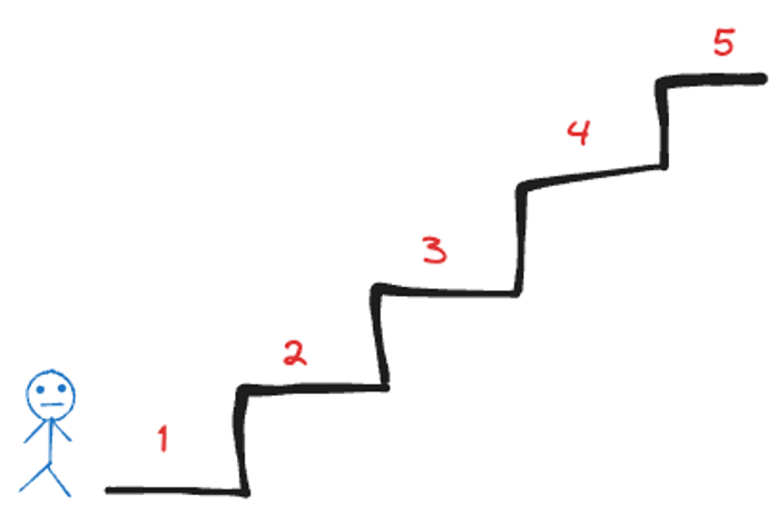"Stairing" into the abyss

From the initial position, you can either go to step 1 or step 2 or step 3.

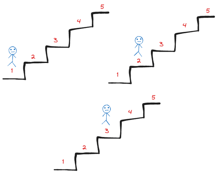The first step (or leap)

Essentially, now the problems breaks down into the sum of three sub-problems:

1. Number of ways you can get to step 5 from step 1. Or, the number of ways you can climb a 4-step staircase (n = 4).
2. Number of ways you can get to step 5 from step 2. Or, the number of ways you can climb a 3-step staircase (n = 3).
3. Number of ways you can get to step 5 from step 3. Or, the number of ways you can climb a 2-step staircase (n = 2).

Mathematically speaking, if the function f(n)f(n)f(n) is defined as the number of ways you can climb a staircase of nnn steps, then:

f(n)=f(n−1)+f(n−2)+f(n−3) f(n) = f(n-1) + f(n-2) + f(n-3) f(n)=f(n−1)+f(n−2)+f(n−3)

A straight-forward code implementation for the same is:

def recursiveSolution(n):
    if n <= 2:
        # When n = 0, 1, 2; return 1, 1, 2 respectively.
        # You can climb a 0 or 1 step staircase in only one way
        # and climb a 2-step staircase in 2 ways ((1, 1) and (2))
        return (1, 1, 2)[n]
    return recursiveSolution(n - 1) + recursiveSolution(n - 2) + recursiveSolution(n - 3)

Tree based approach

Another way that this problem can be approached is by thinking in terms of a tree, where each node of the tree represents your current position on the staircase. There are three possible children from each node, one of every step you can take from your current position.

The tree representation (Download)

Next, you can find all the possible paths to the desired node (position). Each node (position) can be represented by a number, which represents your current position on the staircase. Initially, you start with position = 0 and you need to find all possible paths to position = n (position = 5 in this case).

Tree. Nodes represented as number

This turns into a classic graph/tree problem, which you can solve either by performing a breadth-first search (BFS) or depth-first search (DFS). Implementing a depth-first search would basically replicate the recursive solution implemented earlier, with the only difference being that you would be manually managing the stack, instead of the program managing the stack in the form of call stack. The python implementation of a DFS solution would be:

from collections import deque

def graphDFS(n):
    stack = deque()
    stack.append(0)  # start with position = 0
    count = 0
    while stack:
        x = stack.pop()  # get next position to evaluate
        if n - x <= 2:  # if current position is 0 or 1 or 2
            count += (1, 1, 2)[n - x]  # just add to count
            continue  # further evaluation not needed
        # Append the children to the stack
        stack.append(x + 1)
        stack.append(x + 2)
        stack.append(x + 3)
    return count

The core logic of the recursiveSolution function has been replicated as-it-is to ensure that both functions are as equivalent as possible. The breadth-first version of the solution would be:

from collections import deque

def graphBFS(n):
    count = 0
    queue = deque()
    queue.append(0)  # start with position = 0
    while queue:
        x = queue.popleft()  # get next position to evaluate
        if n - x <= 2:  # if current position is 0 or 1 or 2
            count += (1, 1, 2)[n - x]  # just add to count
            continue  # further evaluation not needed
        # Push the children to the queue
        queue.append(x + 1)
        queue.append(x + 2)
        queue.append(x + 3)
    return count

The two functions are the same except for the usage of stack in one and queue on another. The time complexity of all the three functions is (O(2n))(O(2 ^n))(O(2n)) .

This post assumes that you know how to calculate time complexity. Hence, it does not cover the calculation of the time complexity.

Performance analysis

To benchmark the performance of each of the above functions, I wrote a script that called each function from n = 1 to n = 20 and repeated this x times (called runs). Essentially, I wanted to find the total time taken by a function if it is called for all values between n = 1 and n = 20. The script looks like this:

import time

# Helper function to measure runtime
def measure_runtime(func, n):
    start_time = time.perf_counter()
    result = func(n)
    end_time = time.perf_counter()
    return end_time - start_time, result


function_timings = {}
functions = [recursiveSolution, graphBFS, graphDFS]
times = [0 for _ in functions]  # to store the running times corresponding to each function
runs = 10000  # number of times to repeat the benchmarking => 10, 100, 1000, 10000

for _ in range(runs):
    for n in range(20):  # Test for n = 1 to n = 20
        for i in range(len(functions)):
            func = functions[i]
            time_taken, _ = measure_runtime(func, n)
            times[i] += time_taken

for i in range(len(functions)):
    func = functions[i]
    # Average running time per run
    function_timings[func.__name__] = times[i] / runs

The results shown below is the average execution time per “run”. In other words, each bar shows the total execution time for a function for all values of n from 1 to 20.

As can be seen, clearly the recursiveSolution function is the fastest. The next fastest function is the graphBFS function, which is approximately ~40% slower than recursiveSolution function.

Note

I found it intriguing that graphDFS is the slowest one (even if by a small margin). graphDFS is fundamentally closer to recursiveSolution since both of them use a stack to gather the results.

Thoughts

All the three functions have the same time complexity. All of them essentially implement the same logic. All of them return/continue when number of steps left is less than or equal to 2 (<= 2). Yet, there is a ~40% difference in their performances.

The analysis above aptly demonstrates that equivalent time complexity or algorithmic logic does not necessarily imply equivalent system performance. It is necessary to benchmark the functions/systems we implement to be able to accurately comment on their performance.

However, it would be impractical to benchmark every bit of code we write. The decision on whether or not to benchmark is a judgement call that improves as we learn more about the hidden layers of abstraction in our systems. With knowledge and experience, we can make better judgement on whether or not we use time complexity as the sole metric to gauge the performance of our systems. For example, in almost all cases, binary search would be better than linear search on a sorted list of numbers.

Bonus: Best solution to this problem

The solution to the Climbing Stairs problem that runs in linear time complexity is:

def linear(n):
    a, b, c = 1, 1, 2
    for _ in range(n):
        a, b, c = b, c, a + b + c
    return a

Note

The solution is similar to the solution for getting the nth number in the Fibonacci sequence.

I encourage you to try out different solutions (all of which execute in linear time complexity) and compare their performances. You can compare the above function with this one:

def linear2(n):
    if n == 1:
        return 1
    dp = [0 for _ in range(n + 1)]
    dp[1] = 1
    dp[2] = 2
    for i in range(3, n + 1):
        dp[i] = dp[i - 1] + dp[i - 2] + dp[i - 3]
    return dp[n]

Think about more ways to achieve the same result in linear time complexity and compare their performances.

References

1. CS Primer - Staircase ascent problem → I recommended this course for experienced software engineers who are looking to learn more about the foundational computer science concepts.
2. CS Primer - Seminar on analysing systems

Footnotes

1. Leetcode presents a variant of this problem where you can take only 1 or 2 steps at a time. ↩